Neural Networks are the backbone of AI, particularly in deep learning, in the current age of AI. These networks mimic the human brain making Neural Networks a bundle of nodes linked across several layers to learn to interpret data properly, gradually improving with each layer. However, Graph Neural Networks (GNNs) are underrated despite what a big role it can play in the AI field. Each entity captures information propagating between the layers, producing a better understanding of the data’s complexities for accurate interpretation.
Now, one might ponder “If I barely understand my life let alone my brain, how am I going to understand this system🙄?” Don’t worry—this journey will guide you through the fascinating world of GNNs, step by step👣.
CNN and GNN:
Knowing how important GNNs are, one should initially ask: How did they come to be? What are their foundational principles?
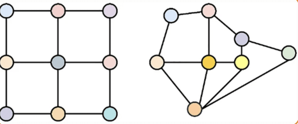
GNNs were heavily influenced from their more famous counterparts, Convolutional Neural Networks (CNNs). While CNNs are designed to work with structured data, like images arranged in a grid, GNNs address a different challenge: unstructured data, such as social networks or molecular structures, where relationships are not arranged in a grid. GNNs use adaptive connections to process complex, irregular data, allowing nodes to exchange information and update their states based on their neighbors. This approach helps GNNs capture intricate patterns in data with flexible structures.
Here is a display of CNNs vs GNNs structures:
Concepts and Architectures:
Simple so far, right? Now let’s take it to another level!
How do GNNs work🤩?
Let us start with G = (V,E) and a history lesson. The graph is set to be made up of two essential parts: V standing for vertices (aka nodes) and E for edges (links). And it is worth mentioning that the graph Laplacian matrix was crucial in developing Graph Neural Networks (GNNs).
When feeding a graph G into a GNN, each node vi is linked with a feature vector xi, and optionally, edges may have feature vectors x(i,j).
The GNN processes these inputs to compute hidden representations hi for nodes and h(i,j) for edges.
GNNs update these representations through a process called message passing:
Edge representations h(i,j) are updated using a function fedge that combines the current node representations hi, hj, with edge features x(i,j): h(i,j) = fedge(hi, hj, x(i,j))
Node representations hi are updated using the fnode function, that aggregates information from neighboring nodes j ∈ Ni (nodes with edges pointing to i) along with the node’s own features xi: h’i = fnode(hi, {hj | j ∈ Ni}, xi) Here, Ni denotes the set of neighboring nodes of i.
These updates are iterative, allowing nodes to refine their representations through multiple rounds of message passing. GNNs like the Graph Convolutional Network (GCN) generalize and combine previous models by using shared parameters in fedge and fnode.
This approach extends principles from recurrent neural networks to graph data.
And yes, equations can look intimidating, but remember, even Allen Iverson had his own way of saying, “Now we talking about equations…? Really, equations?” Keep calm and crunch the numbers!
Techniques and Challenges:
To effectively use Graph Neural Networks (GNNs), it’s crucial to understand their reliance on message passing, where nodes update their representations based on neighboring nodes. Multi-Layer Perceptrons (MLPs) are often employed to refine these data sets. However, several challenges persist:
Scalability: Processing vast amounts of graph data, like that on Twitter or X with millions of nodes and billions of edges, presents a significant challenge. This requires specialized hardware and efficient algorithms due to the limitations of traditional GPUs and the need for low latency.
Interpretability: Understanding graph visualizations varies widely depending on one’s background and goals. This often leads to differing interpretations, highlighting the gap between technical and non-technical perspectives.
Dynamic Graphs: Graphs that evolve over time with changing nodes and edges introduce additional complexity. Different types of dynamic graphs each come with their own set of advantages and limitations.
As The Rock might put it, “We’re laying the smack down on these challenges—one update at a time!”
Graph Based Tasks:
Graph-based tasks vary depending on their focus and can be divided into three main categories:
Node Level Tasks: These involve classifying, clustering, or predicting properties of individual nodes. For instance, in financial networks, tasks might include assessing the legitimacy of transactions based on their connections.
Edge Level Tasks: These focus on relationships between nodes, such as determining whether a link exists or predicting interactions. An example is recommending products based on user behavior patterns.
Graph Level Tasks: These analyze entire graphs to perform classification, regression, or coordination. In drug discovery, for example, GNNs help in understanding molecular structures, with nodes representing atoms and edges representing chemical bonds.
Graph Variants:
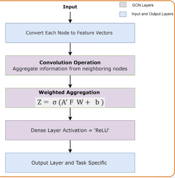
Inhale and exhale young padawans for the force is strong with you. Graph Convolutional Networks (GCNs) are an evolution of graph neural networks that utilize the Laplacian graph. They operate by having neighboring nodes aggregate data through a weighted sum of their feature vectors. The weights are distributed according to the normalized adjacency matrix, resulting in new vectors for each node.
This process is captured in the equation Z = σ(A’FW + b),
where:
Z is the output,
σ is the activation function (think of ReLU as your trusty lightsaber),
A′ is the transpose of the adjacency matrix,
F is the feature matrix,
W is the weight matrix, and
b is the bias vector.
This setup prepares the model for application of a non-linear activation function like ReLU.
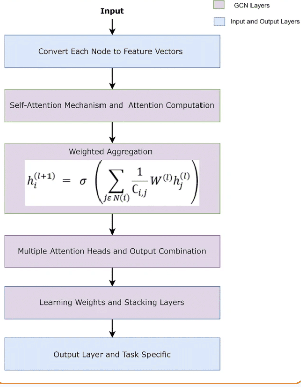
GATs: The Attention Seekers of the Graph World
Unlike their predecessors, GATs allow each node to have its own weight, determining how much it influences its neighbors. This dynamic weighting lets the network adapt and fine-tune its connections in real time.
The process is elegantly captured by this improved equation:
hi(l+1) = σ(Σj∈N(i) 1/Ci,j W(l)hj(l))
where:
hi(l+1): The updated feature vector of node i at the (l+1)-th layer.
σ: An activation function, typically a non-linear function such as ReLU.
Σj∈N(i): The summation over all neighbors j of node i in the set N(i).
1/Ci,j: A normalization constant that accounts for the degrees of nodes i and j.
W(l): The weight matrix at the l-th layer, which is learned during the training process.
hj(l): The feature vector of the neighboring node j at the l-th layer.
GATs make GCNs look like they’re playing with training wheels!
With the evolution of GNNs, many variants have emerged, each adding its unique twist:
Directed Graph: has edges with direction, indicating specific relationships between nodes, such as a parent-child relationship in a class hierarchy.
Heterogeneous Graph: includes various types of nodes and uses techniques like one-hot encoding for standardization, with methods like Graph Inception and Heterogeneous Graph Attention Networks to handle these diverse characteristics.
Dynamic Graph: has adaptable structures where nodes and edges can change over time, supporting algorithms that evolve with new data.
Attributed Graph: carries additional data on edges, such as weights or types, enhancing models like G2S encoders and Relational-GCNs to better manage node relationships.
Conclusion:
Graph Neural Networks (GNNs) are powerful tools for handling graph-structured data, allowing them to capture complex relationships and dependencies within datasets. Initially inspired by simpler concepts, GNNs have evolved to tackle a wide range of tasks, including node classification, link prediction, and graph-level prediction. Their versatility is evident in applications such as social network analysis, recommendation systems, and drug discovery.
So, while GNNs might not wear capes, they sure do a lot of heavy lifting🏋️ —and make data analysis look pretty cool.